In this article, I’ll describe the necessary steps to accomplish most LUT creation tasks in Blackmagic Design Fusion.
Contents
- What are LUTs?
- LUT tools in Fusion
- Visualizing your LUTs in Fusion
- Examples
- Authoring 3D LUTs
- Authoring 1D LUTs
- Convert a 3D LUT to a 1D LUT
- LUT Smoothing
- Compositing LUTs together
- Color Spaces and LUTs
- Resize a LUT
- Make a monochrome version of a LUT.
- Create an identity LUT
- Change the grayscale behavior of a LUT
- Adjusting the LUT for Video Levels
- Make an exposure compensation LUT.
- Make a Linear to Log 1D LUT
- Conclusion
What are LUTs?
For this article, consider a color pipeline that has no spatial operations. IE, every RGB pixel in the image is given the same function, regardless of its position in the image. Let us call this function \(f: \mathbb{R}^3 \rightarrow \mathbb{R}^3\). This takes Red, Green, and Blue code values as input and outputs a new set of Red, Green, and Blue code values. Sometimes it makes sense to bake this function \(f(r, g, b)\) into a LUT so that it can be quickly evaluated, or to obfuscate the math used to make it. This article will discuss Cube LUTs.
LUT is short for “Look Up Table”. Our RGB color pipeline is evaluated at regular intervals between some minimum input (the DOMAIN_MIN, which defaults to \((0, 0, 0)\)) and some maximum input (the DOMAIN_MAX, which defaults to \((1, 1, 1)\)). These Min and Max tags can be specified to override the default values, but they rarely are used in practice. The size of the LUT controls the sampling frequency and is specified by a tag called LUT_1D_SIZE or LUT_3D_SIZE, for 1D and 3D LUTs respectively.
If we consider a 1D LUT with the tag LUT_1D_SIZE 65 specified, the table will consist of 65 rows. The rows will be calculated in the following way:
A 3D LUT with the tag LUT_3D_SIZE 65 will consist of \(65^3\) rows, which will be ordered in the following way:
Above, the red channel iterates through all 65 samples most rapidly, then green, then blue iterates the slowest.
When the LUT is evaluated on an image, we first fetch the \((r, g, b)\) code value for each pixel in the image. Each channel of the \((r, g, b)\) code value is clamped to the DOMAIN_MIN to DOMAIN_MAX bounds. Next, we look up the closest entries in the table for that code value triplet.
For a 3D LUT, the nearest eight points to the \((r, g, b)\) coordinates are identified and interpolated ideally using tetrahedral interpolation. For a 1D LUT, it is assumed that the three channels are independent:
\[\text{assume} \; f(r, g, b) = f_r(r), \; f_g(g), \; f_b(b)\]We then sample the two closest values in the table for \(f_r(r), f_g(g), f_b(b)\) to the input pixel’s code value. We will then use a simple Linear interpolation between these values to get the code value for each channel.
As an example for 1D LUTs, I have created a strong S curve that we will apply with a LUT size set to 8, 16, 32, and 64 points.
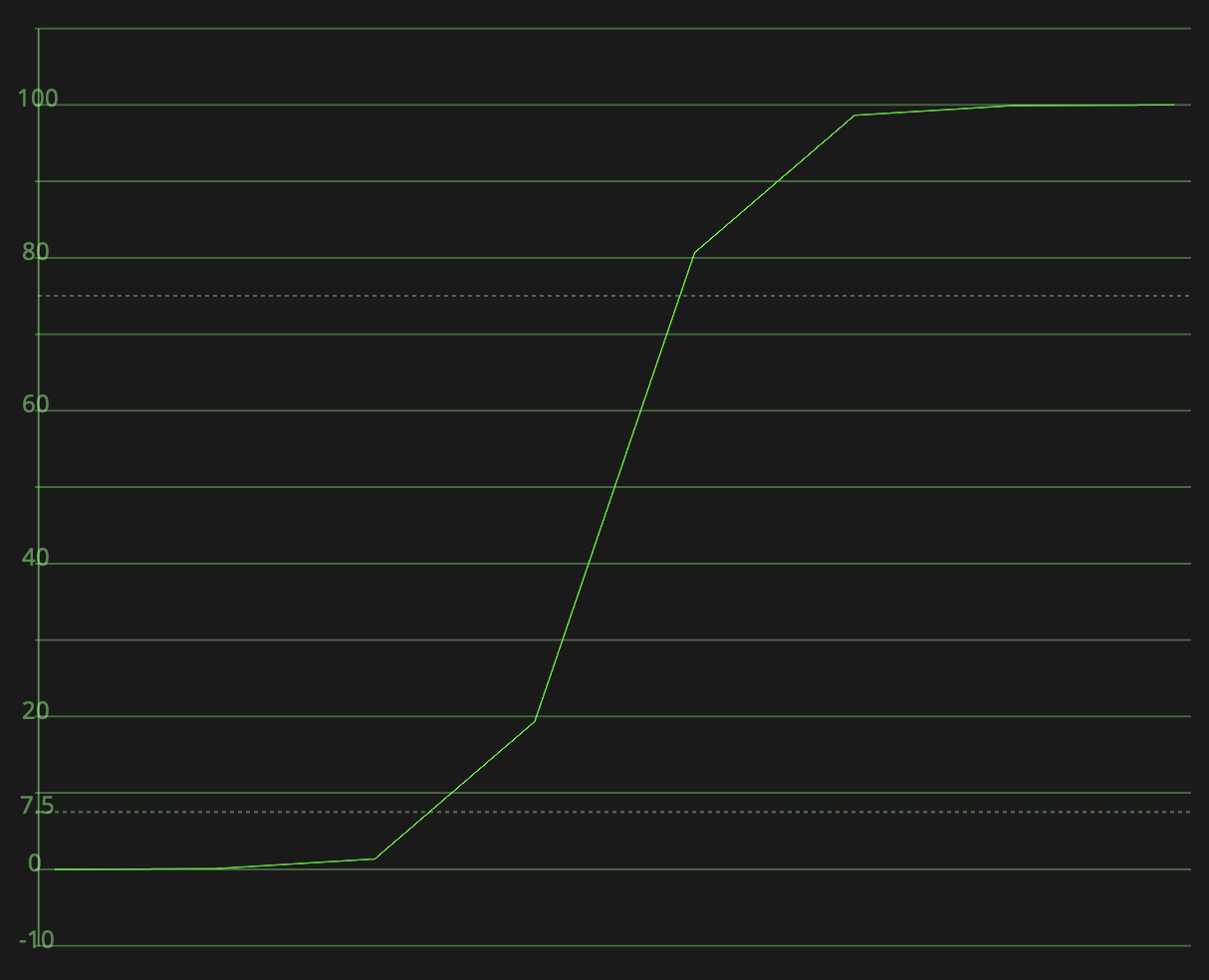
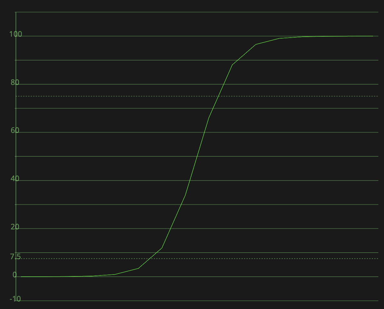
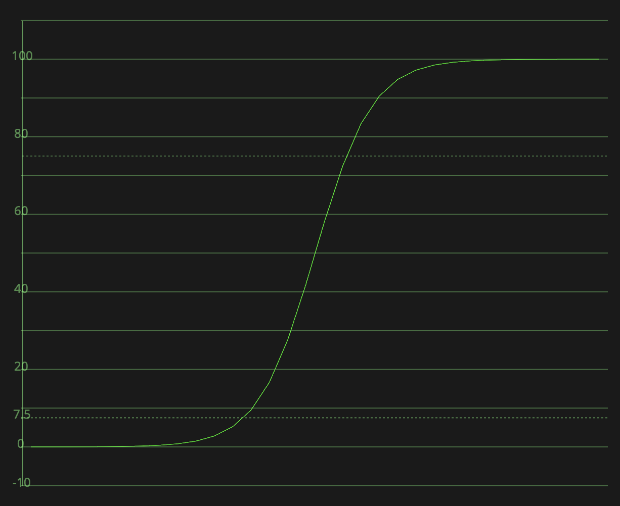
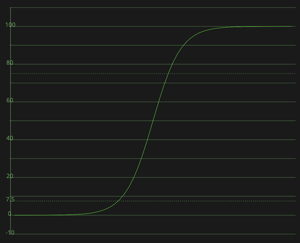
Takeaways
- Increasing the size of the LUT will reduce the interpolation error.
- Having a LUT size that’s too low will result in both inaccuracy and a less smooth function.
- The visual impact of the interpolation error is dependent on the function being sampled, the incoming code value, and how it’s being used.
- LUTs clamp off inputs that are outside their
DOMAIN_MINandDOMAIN_MAXdomain, which makes them inappropriate for use on images with negative values or code values above 1.0. - LUTs are uniformly sampled, which generally makes them inappropriate for use on linear domain images.
LUT tools in Fusion
3D LUTs
Fusion comes built-in with a handful of effects for manipulating LUTs:
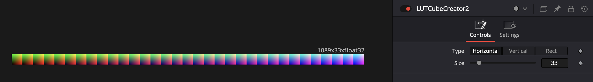
LUTCubeCreator
This tool generates an image that contains a pixel for each row that will exist in a 3D cube LUT of a given size. This is sometimes called a “HALD Image”
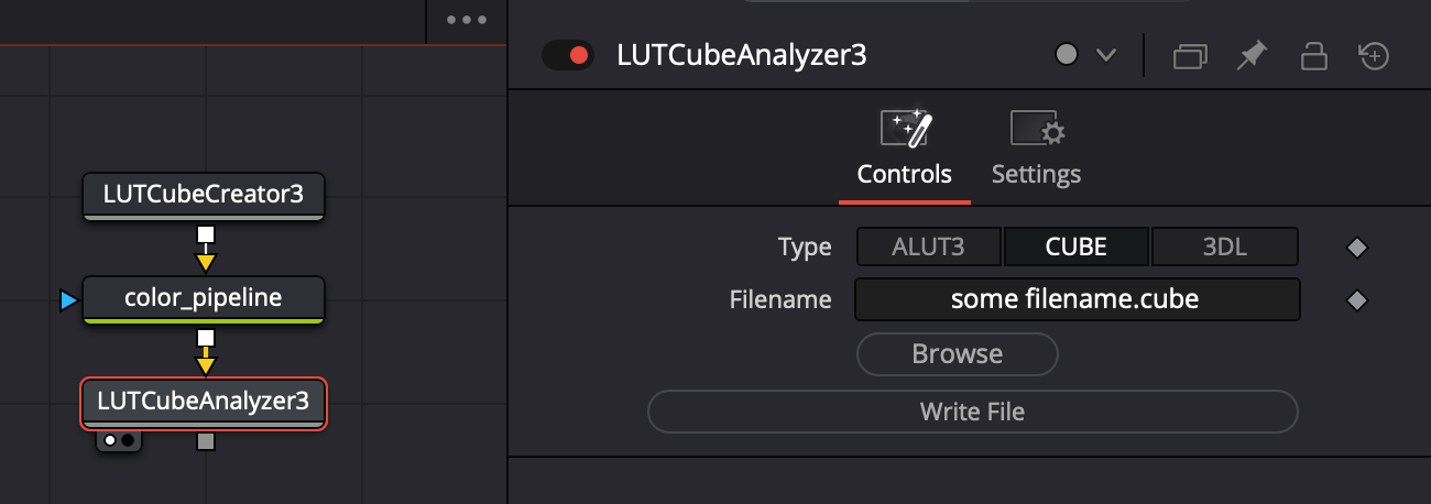
LUTCubeAnalyzer
This is a tool that should be given a HALD Image of the same shape as those outputed by LUTCubeCreator, and writes it to disk as a LUT in one of a few different formats. Once a HALD image is connected as the input to this node, you simply choose a location to save the LUT, and then click “write file”.
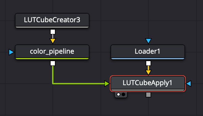
LUTCubeApply
This Fusion tool takes a HALD image of the same shape as outputted by the LUTCubeCreator as the foreground and applies it to the image in the background. It uses linear interpolation instead of tetrahedral interpolation.
1D LUTs
For manipulating 1D LUTs, I’ve made a series of fuses that you can download and install for Fusion below, by navigating to the Fuses folder.
LUTCubeCreator1D
Similarly to the 3D version, this creates a horizontal image of a 1D LUT. 1D LUTs are much for space efficient for a given side (due to the number of rows being equal to the size rather than the cube of the size) and therfore you can safely set this to a larger number lik 4096.
LUTCubeAnalyzer1D
Similarly to the 3D version, this allows you to write 1D LUTs to either a Cube or SPI1D format. The latter is often used by OCIO configs.
LUTCubeApply1D
Applies a 1D LUT, similarly to the 3D version. Also allows you to unclamp the LUT, which linearly extends the first and last two rows in the table.
Applying LUT files
There are multiple ways to apply a LUT that has already been written to a .cube file or other file type
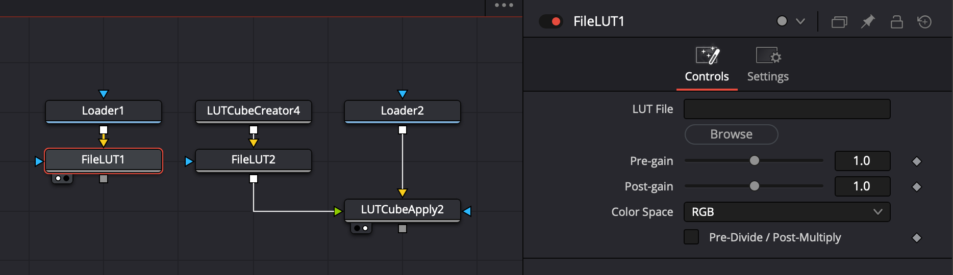
FileLUT
This allows you to apply a 1D or 3D LUT file to an image. This uses linear interpolation.
OCIOFileTransform
This allows you to apply a 1D or 3D LUT file to an image, and lets you choose linear or tetrahedral interpolation. Also allows you to invert a loaded 1D LUT by choosing “Reverse” as the direction.
Visualizing your LUTs in Fusion
LUT Behavior on a grayscale
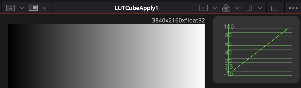
You can see what your LUT does to a gray ramp with the following chain of nodes:
- Background node, set the “Type” to Horizontal and make a gradient from \((0, 0, 0)\) to \((1, 1, 1)\).
- OCIOFileTransform node to apply your LUT, if it’s already written to a file. Otherwise use LUTCubeApply or LUTCubeApply1D.
You’d then send node (2) to one of the viewers and click the “SubView” button in the top left corner of the viewer (highlighted below). You can change the type of visualization to Waveform. Right clicking on the waveform subview that appears allows you to change settings of the visualization, such as if you want to switch to RGB mode or change the sampling.
Another option is this:
- Background node, let as black
- Apply my Exposure chart DCTL, whose download link is below
- ColorSpaceTransform from Linear to your LUT’s expected input color space
- OCIOFileTransform to apply your LUT.
This would give you the behavior of the LUT in one-stop increments.
LUT Behavior as a cube
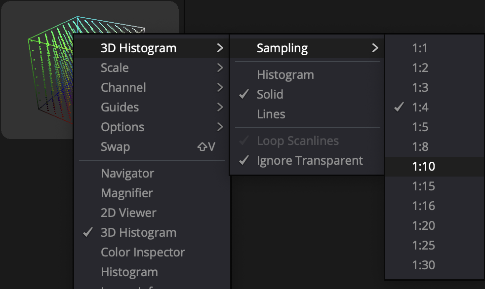
Use the following chain of nodes:
- LUTCubeCreator, set to some size
- OCIOFileTransform node to apply your LUT, if it’s already written to a file. Otherwise use LUTCubeApply or LUTCubeApply1D.
Sending node (2) to one of the viewers, similarly to the previous section, you would then click the SubView button, right click on the scope and choose “3D Histogram”. I prefer to set it to Solid and choose something reasonable for the sampling frequency; note that on full sized HD or 4k images, Fusion will run quite slowly if your sampling frequency is too high.
Examples
Below I will outline some example use-cases and how to implement them in Fusion.
Authoring 3D LUTs
You can easily make 3D LUTs in Fusion with the following chain of nodes:
- LUTCubeCreator, set to the size that you wan the 3D LUT to be
- Whatever color grade or operations you want to bake into a LUT
- LUTCubeAnalyzer, to save the 3D LUT to a .cube file. Simply choose a location and then click “Write File”
This written file from (3) can be applied to an image using FileLUT, or preferably OCIOFileTransform, which supports tetrahedral interpolation. Alternatively, you can also use LUTCubeApply to apply the HALD image as a LUT.
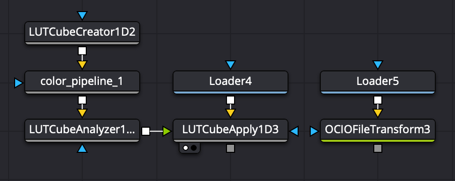
Authoring 1D LUTs
We can create and apply 1D LUTs through the following chain of nodes
- LUTCubeCreator1D, set to the size of your preference
- Whatever color grade or operation you want to capture in the 1D LUT.
- LUTCubeAnalyzer1D, to save the 1D LUT to a file.
The written file from (3) can then be applied to an image using FileLUT or OCIOFileTransform. Alternatively, you can use LUTCubeApply1D.
Inverting a 1D LUT
You can load a 1D LUT into OCIOFileTransform and click Reverse as the direction.
Convert a 3D LUT to a 1D LUT
Set up the following chain:
- LutCubeCreator1D, set to the size you want the 1D LUT to be.
- OCIOFileTransform, load up the 3D LUT you’re concerned about and set the interpolation to tetrahedral
- LUTCubeAnalyzer1D, to save the 1D LUT somewhere
LUT Smoothing
Sometimes you want to smooth out a LUT, to remove any hard creases in the LUT. Before starting, be sure to download my LUT Smoother fuse here:
- LUTCubeCreator, in “Horizontal” mode, set to the size of your choice (presumably the size of the LUT that you’re trying to smooth)
- LUTSmoother fuse, set to blur the achromatic and saturated parts of the cube as desired
- LUTCubeAnalyzer, to write the resulting LUT to a file
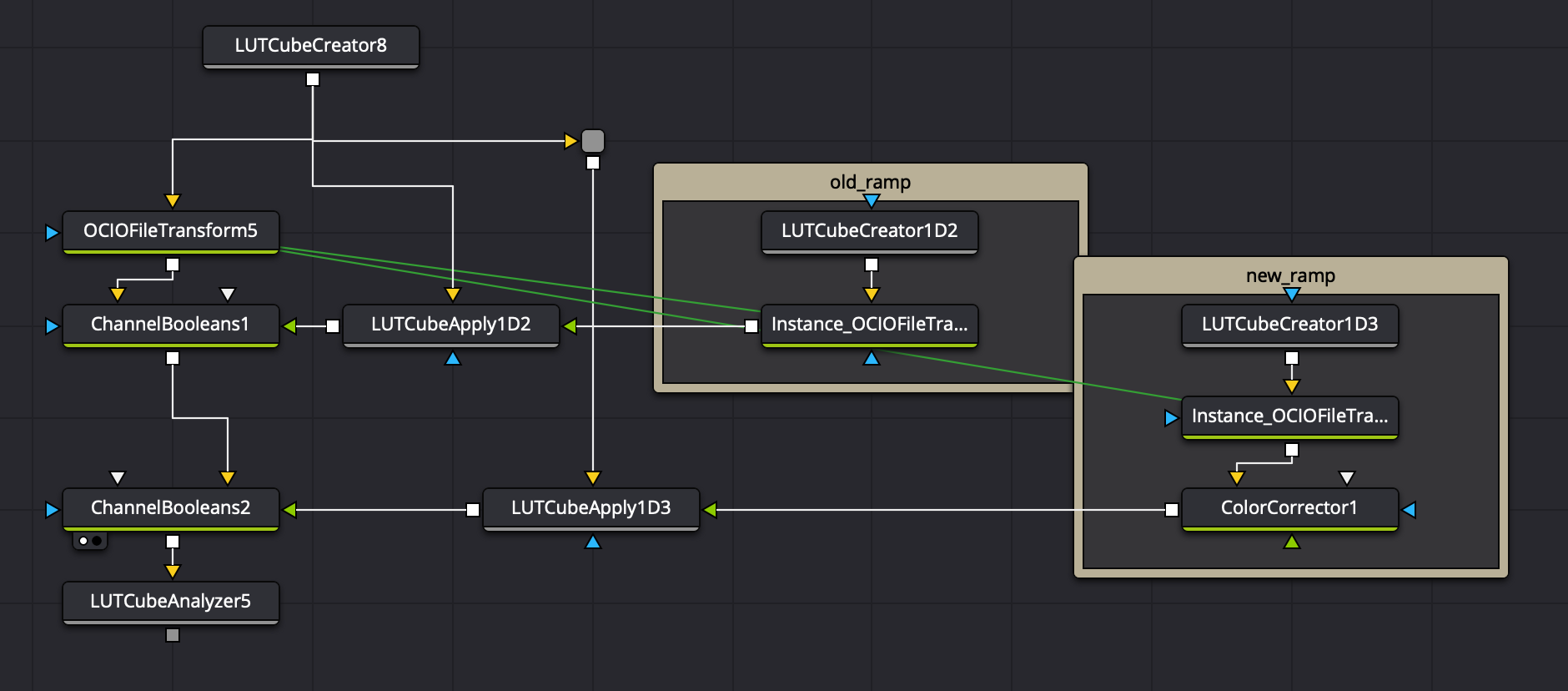
Compositing LUTs together
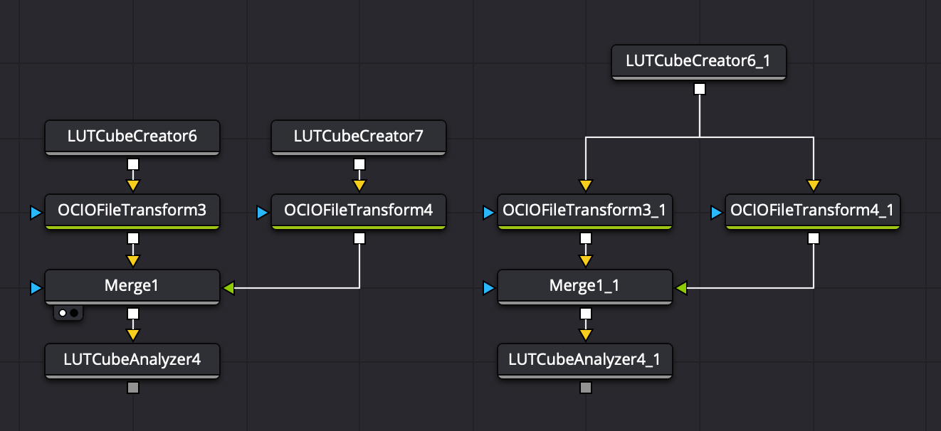
Sometimes you may want to grab the “colors” of one LUT and the “contrast” of another LUT. Here’s one approach to doing that.
- Create a LUTCubeCreator node in the size that you want to output
- Apply the color pipeline you want to extract the “colors” from, say, with an OCIOFileTransform set to Tetrahedral mode
Repeat the above two steps in a separate chain for the LUT or pipeline you want to extract the “contrast” from.
- Create a Merge node where the background is fed by the “Contrast” HALD image and the foreground is fed by the “Color” HALD image. Set the “Apply Node” for this merge node to “Color”
- Send the output of the Merge node to a LUTCubeAnalyzer to save the resulting cube LUT somewhere.
You can follow the approach in either of the below graphs.
Color Spaces and LUTs
Suppose you have a LUT that expects one color space but you want to use it on an image in a different color space. Create the following chain of nodes.
- LUTCubeCreator, in the size of the LUT that you want to output
- ColorSpaceTransform, from the color space of the image to the expected color space of the LUT
- OCIOFileTransform or FileLUT node to apply your LUT.
- (Depending on your use-case) Another ColorSpaceTransform to go from the LUT’s output color space to another color space if you’d prefer.
- LUTCubeAnalyzer to save the resulting LUT somewhere
Resize a LUT
Some monitors don’t support LUTs over the size of 33 points, so you may want to take an existing 65 point LUT and scale it downwards using the following chain:
- LUTCubeCreator, set to the size you want to output (33 in this example)
- OCIOFileTransform to apply your larger LUT with tetrahedral interpolation
- LUTCubeAnalyzer, to save the reduced size LUT somewhere.
Importantly, note that if you try to resize a LUT to be larger, you will not really gain any significant smoothness or accuracy advantages, compared to having authored the LUT in the larger size in the first place.
Make a monochrome version of a LUT.
Simply put, apply the following chain:
- LUTCubeCreator, set to the size you want to output.
- OCIOFileTransform to apply your colorful LUT
- The desaturation operation of your choice (ColorCorrector node or perhaps the ColorMatrix node, etc.), lowering the saturation towards zero.
- LUTCubeAnalyzer, to save the desaturated LUT somewhere
Create an identity LUT
Suppose you want to make a LUT that doesn’t do anything. You’d create the following chain of nodes:
- LUTCubeCreator, set to the desired output size
- LUTCubeAnalyzer, to save this LUT.
Change the grayscale behavior of a LUT
Suppose you want to replace the grayscale behavior of one LUT with another’s.
- LUTCubeCreator in the desired LUT size.
- OCIOFileTransform, to apply the LUT you want to modify
- ChannelBoolean, set to Subtract (and Alpha set to Do Nothing)
- ChannelBoolean, set to Add (and Alpha set to Do Nothing)
- LUTCubeAnalyzer, to save the resulting LUT somewhere
In the foreground of (3), you must pipe in a LUT that has the grayscale behavior/1D curve you want to remove from the LUT:
- LUTCubeCreator in the same LUT size as before
- 1D curve that captures the behavior of the LUT that you want to remove.
- The foreground here could be generated via LUTCubeCreator1D, followed by an OCIOFileTransform of the LUT you wanted to modify, set to tetrahedral interpolation.
Similarly, in the foreground of (4), you will pipe in the grayscale behavior/1D curve that you want to add to the LUT:
- LUTCubeCreator in the same LUT size as before
- 1D curve that captures the behavior of the LUT that you want to add.
- The foreground here could be generated via LUTCubeCreator1D, followed by whatever method you want to use to create a new 1D curve. In the below example, we suppose that I wanted to remove the split tone and I used a ColorCorrector to reduce saturation
Alternatively, you could play with inverting the curves you want to remove and then applying the curve you’d rather have.
Adjusting the LUT for Video Levels
Some monitoring systems apply a LUT without first scaling the signal from video to full levels. If you have one of these, you’ll need to modify the LUT accordingly to get the right contrast in your image. First, you’ll need to download my Levels Conversion DCTL and then apply the following chain:
- LUTCubeCreator in the desired output size
- Levels Conversion DCTL to go from the levels that the system offers to the LUT, to the levels expected by the LUT
- OCIOFileTransform in tetrahedral mode to apply the LUT
- (Might be required) Levels Conversion DCTL to go from the levels that the LUT outputs to the levels the system expects from the LUT.
- LUTCubeAnalyzer, to save the LUT somewhere.
Make an exposure compensation LUT.
Sometimes it’s helpful to have a monitoring LUT that includes a one stop overexposure recommendation. This can easily be done, supposing that you already have a LUT that goes from the camera log space to Rec709. You’d use the following chain:
- LUTCubeCreator, set to the size that you want for your LUT.
- ColorSpaceTransform from your camera’s log curve to linear, with no OOTF boxes checked nor tone mapping/gamut mapping.
- ColorGain node to apply a gain/exposure adjustment. Set this to \(2^x\) where \(x\) is the number of stops you want to compensate for. IE if you want the user to overexpose by one stop, set this to 0.5.
- ColorSpaceTransform from Linear to the camera’s log curve, with no OOTF boxes checked nor tone mapping/gamut mapping.
- Your normal LUT or pipeline used to make the normal LUT
- LUTCubeAnalyzer, to save the LUT to a file somewhere.
Make a Linear to Log 1D LUT
Unlike the other ones, this is a multi-step process. First we must identify the white point of a log to linear conversion using the following pipeline.
- Background node set to \((1, 1, 1)\).
- ColorSpaceTransform from the log cuve of your choice to Linear, with no forward OOTF nor tone mapping.
- Measure this white point and call it \(W\). It will typically be larger than \(1.0\).
We will repeat the process with the black point.
- Background node set to \((0, 0, 0)\).
- ColorSpaceTransform from the log curve of your choice to Linear, with no forward OOTF nor tone mapping.
- Measure this black point and call it \(B\). It can be negative.
If you want, you can also choose arbitrary values of \(B\) and \(W\). I have had success choosing something like \(B = -1.0\) and \(W = 100.0\) for a Linear to LogC3 LUT. It may be recommendable to play with the LUT sampling when you do this.
Then, make the following chain of nodes:
- LUTCubeCreator1D, set to the size of your choice (ideally at least \(2^{12}\)).
- ColorGain node, with Gain set to \(W\) and lift set to \(B\).
- ColorSpaceTransform from Linear to the log curve from before.
- LutCubeAnalyzer1D, to save the LUT to a file somewhere.
You will then open the resulting LUT file and add the following line to the top:
LUT_1D_INPUT_RANGE <B> <W>
As an example, it might look like this:
LUT_1D_INPUT_RANGE 0.0 38.42093
If the above doesn’t work, then it’s probably because your software expects the official adobe tags DOMAIN_MIN and DOMAIN_MAX, rather than the above tags which are expected by Resolve. The above lines would instead look like:
DOMAIN_MIN 0.0 0.0 0.0
DOMAIN_MAX 38.42093 38.42093 38.42093
Conclusion
Given the capabilities of Fusion, I personally see little reason to buy other programs for manipulating LUTs. Using the methods described in this article, you should be able to generalize to your own use-cases.